

This is part seven of a series that I think we’ve all lost interest in but which I’m determined to finish.1 As always, here’s the seed and what has gone before:
A Formula for Meaningful Complexity, by
.This series: Part 1, Part 2, Part 3, Part 4, Part 5, and Part 6.
Obviously, all are required reading for this post.2
Without further ado, here we go…
Blanking versus Randomizing an Image
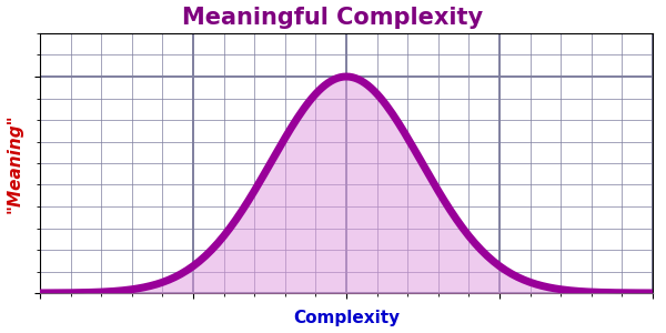
A key part of the ESC calculation3 is the EF (Emergence Factor):
Which looks complicated but is fairly simple when considered as just the A/B ratio where A is the area below the curve, and B is the area above it — both areas limited by the upper and lower extent of said curve. (See Part 2 for details.)
Previous calculations of the EF assumed a series of images or texts that began with the image or text and progressively added noise to make the last image or text of the series 100% randomized. Now we’ll consider an idea discussed in the first post: a progression of images (or texts) from blank to the image (or text) and then to random noise.

As discussed previously, we only have one useful path to full randomization — “full spectrum” (i.e. 8-bit) noise. But as noted in Part 4, we have multiple options for how we “blank” a file. In particular, we can replace some percentage of pixels with a solid color (white, gray, or black), or we can fade all pixels some percentage towards white, gray, or black.
Note that since Part 4 I’ve added a noise mode. Here’s the updated list:
Mode 0: Replace X% of pixels with random colored pixels.
Mode 1: Replace X% of pixels with random grayscale pixels.
Mode 2: Replace X% of pixels with black pixels.
Mode 3: Replace X% of pixels with 50% grey pixels.
Mode 4: Replace X% of pixels with white pixels.
Mode 5: Fade all pixels X% towards black.
Mode 6: Fade all pixels X% towards gray.
Mode 7: Fade all pixels X% towards white.
Mode 8: Fade all pixels X% towards random color.
Mode 0 is the full spectrum image noise used in all previous examples. Mode 1 and Mode 8 are alternate noise modes that weren’t effective and aren’t used. Mode 0 gives us the type of compression curve we’ve seen before:
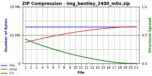
The (green) curve begins with the level of compression for the original image — presumably the most the image can be compressed — and declines towards the zero compressibility of a 100% randomized image.
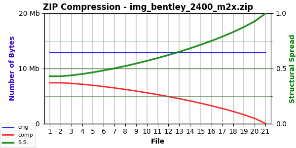
Modes 2, 3, and 4 replace a percentage of pixels. Modes 5, 6, and 7 fade the image by changing all pixels by a percentage.4 These two styles of blanking reverse the compression curve because the blank image (the final state) is highly compressible in contrast to the final incompressible 100% randomized state.
So, while above the green curve drops to zero, in the blanking modes, it again starts at the compressibility of the original image but then rises to close to 100%. Here’s the blanking curve for Mode 2:
And here’s a nearly (but not quite) identical curve for Mode 5:
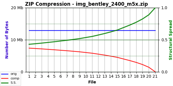
Fading the image seems to give a deeper curve (one with more curvature) than replacing pixels, and it’s possible that the difference between them says as much about the image structure as does anything we’ve seen so far.
Both modes above blank to a black image. Blanking to a white image gives identical curves, but blanking to gray gives a very slightly different one. It’s only visible on the graphs by blinking back and forth between, but it shows up better in the numbers.
For the “Bentley” image, with 2400×1800 resolution, the SS value for Modes 2 through 7 is extremely high: 0.99793 in all six cases (only varying in the sixth decimal digit). But the EF values differ, both between black/white versus gray, and between pixel replacement (Modes 2-4) versus pixel fading (Modes 5-7).
Here are the EF (and ESC) values for compression curves using these modes:
Mode 2 (black): 1.814375 (27,610.37)
Mode 3 (gray ): 1.842391 (28,044.05)
Mode 4 (white): 1.817091 (27,657.15)
Mode 5 (black): 2.261783 (34,418.79)
Mode 6 (gray ): 2.280044 (34,705.75)
Mode 7 (white): 2.255435 (34,328.93)
Firstly, a stark difference between the two groups. The EF is about 1.8 for replacement and 2.2 for fading. Secondly, the black and white modes are close to identical whereas the gray modes have distinctly higher EF values.5
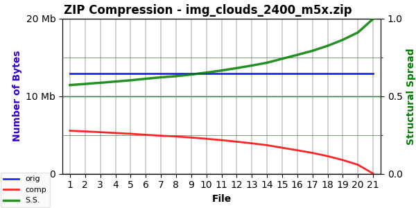
The other camera images have similar differences. For example, “Clouds” is one of the simpler ones. Its Mode 0 curve has an SS of 0.571971, an EF of 1.603331, and an ESC of 5,087,182. Using the blanking modes, as expected, the SS values are very high and nearly similar — 0.997 (with variance in the fourth decimal digit). But the EF (and ESC) values again differ:
Mode 2: 2.038527 (31,001.73)
Mode 3: 2.058831 (31,318.68)
Mode 4: 2.039740 (31,026.26)
Mode 5: 2.269572 (34,513.57)
Mode 6: 2.311152 (35,155.07)
Mode 7: 2.263934 (34,434.59)
Low ESC values due to the extreme compression of the fully blank image. Again, a definite difference between the two groups and elevated values for the gray modes (3 and 6). These EF values are higher than for the Mode 0 curve. Here’s the chart for Mode 5:
On the other end of the spectrum, the very complex “Trees” image. The randomized version had a low SS of 0.062774 with an EF of 2.598041 (both indicating considerable fine structure). With the blanking modes:
Mode 2: 1.390425 (21,175.97)
Mode 3: 1.389857 (21,172.86)
Mode 4: 1.392688 (21,214.61)
Mode 5: 2.843105 (43,300.08)
Mode 6: 2.869583 (43,714.79)
Mode 7: 2.837888 (43,229.12)
But now the pixel replacement with gray has a lower EF whereas fading to gray still has a higher one. Still a difference but in opposite directions. I think this might be significant but haven’t figured out what it’s saying.6
Here is the chart for Mode 5:
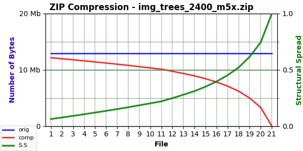
Which is interesting in running from the extremely low compressibility of the original image to the extreme compressibility of the blank image.7
On the other end of that spectrum, the Mode 2 curve for the flag of Norway (a very simple image) surprised me:
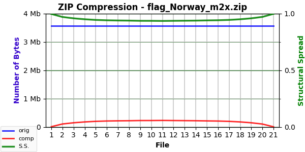
Until I figured out what was happening. The Mode 5 curve was even more surprising:
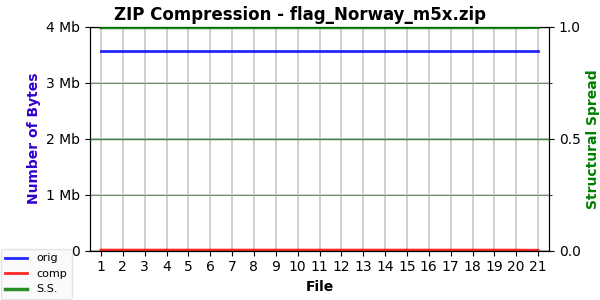
Flatlines! Or nearly so. Fading a sufficiently simple image to a solid color (be it black, gray, or white) results in extremely compressible outputs throughout the process. The original image (flag of Norway) compresses to 0.2107% (⅕ of one percent). As the image fades to black, that drops imperceptibly to 0.2085% at 95% black. That remaining 5% clearly provides a tiny bit of structure, because the final 100% black image compresses to 0.1187%.
The shallowness of the above curve for “Clouds” (a fairly simple photo image) is a step towards this flatness. Here’s the Mode 2 compression curve for “Mandelbrot 2” (see Part 4):
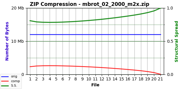
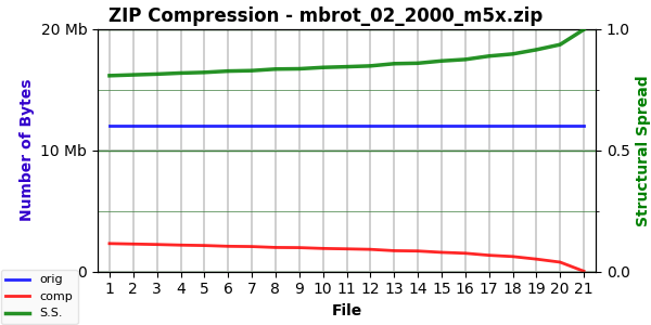
That image is simple enough to have a high compression value (left end of green curve). Blanking it with pixel replacement at first makes it slightly less compressible, but it soon turns the other way. In contrast to more complex images, the Mode 5 curve here has less curvature:
The bottom line, as is so often the case, is that “it depends.” I decided to look at both Mode 2 and Mode 5 as blanking modes (and, of course, Mode 0 as the randomizing mode). Comparing the two seems meaningful. There is no significant difference in blanking to white, to gray, or to black.
Substack is whining about post length, and rather than put up with the whining, I’ll end here in hopes of kicking out several more (shorter) posts very soon.
In the next post(s) I’ll discuss the results of “crossfading” an image from 100% blank (black in these examples) to the image and then to 100% random noise.
Until next time…
Not, I like to believe, because of a sunk cost fallacy but because the job isn’t over until the paperwork (documentation in this case) is done (even though it’s never as much fun as the project itself).
Unless you just like looking at graphs and numbers.
Which, recall, is:
Where AC (Actual Compression) is the minimum size and SS (Structural Spread) is a measure of compression. See Part 2 for details.
Part 4 has example images of all modes with 50% noise. (Except that, because Mode 6 was inserted later, there is no example image, and Modes 6 and 7 are now Modes 7 and 8.)
The randomized version of the same image has an EF of 1.763179.
Of note is that the more complex the image, the greater the difference between the two mode groups.
Hence the high EF value of 2.8.