The Bloch Sphere

A handy way to visualize the quantum states of spin ½ particles (or light polarization).

The Bloch sphere labeled with the canonical |0⟩ and |1⟩ states.

In quantum computing, where qubits are central, the Bloch sphere is useful for depicting two-level quantum systems (i.e. a qubits). As I mentioned last time, it’s also useful for particles with a quantum spin of ½.¹

This post assumes you’re familiar with the material covered last time:

Quantum Spin

The idea dates back to 1892 when Henri Poincaré defined the Poincaré sphere to describe all possible states of light polarization² — linear, circular, and elliptical (a topic for another time).

Defining the Bloch Sphere

The Bloch sphere labeled with its canonical 3D axes.

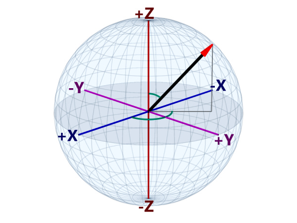
The three-dimensional Bloch sphere has X, Y, and Z axes. Each axis intersects the surface of the sphere at two antipodal points (opposites sides of the sphere — see images above). Together, they define six points on the sphere — the six canonical eigenstates of spin ½ particles.³

The surface of the Bloch sphere is the set of all pure quantum states of the system — states which can be defined in terms of any eigenbasis on the sphere. (The interior of the sphere is the set of all mixed quantum states.)⁴

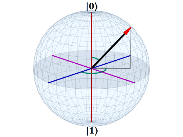
As is common in geometry, we simplify the math by taking the sphere to have a radius of 1. We imagine a unit vector — the black arrow in these images — that represents the quantum wavefunction at a given moment. This vector moves smoothly around the sphere as the wave-function evolves over time per the Schrödinger equation. If the system is measured, however — causing wavefunction “collapse” — then the vector jumps instantly to a new state due to the measurement.

For more details about measurement, see:

The Vexing Problem of Wavefunction Collapse

Bloch Sphere Eigenstates

The Bloch sphere labeled with its canonical eigenstates along with the superpositions that define the |+⟩, |-⟩, |i+⟩, and |i-⟩ eigenstates.

A spin or qubit measurement can have two outcomes, sometimes labeled |0⟩ and |1⟩ (“ket zero” and “ket one”). These are at the north and south poles of the sphere, respectively. This polar axis (dark red) is canonically defined as the Z-axis.

For more details on “kets” (and “bras”) see:

Bra-Ket Notation

A vital point here is that antipodal points, such as |0⟩ and |1⟩ are orthogonal states. Often in geometry, orthogonal means lines that meet at a 90° angle, but in the Bloch sphere we define orthogonal as a 180° angle.⁵

We define the |0⟩ and |1⟩ vectors as:

\(|{0}\rangle\!=\!|{Z}_{+}\rangle\!=\!\!\begin{bmatrix}{1}\\{0}\end{bmatrix},\quad |{1}\rangle\!=\!|{Z}_{-}\rangle\!=\!\!\begin{bmatrix}{0}\\{1}\end{bmatrix} \)

For these to be orthogonal, their inner product must be zero, and sure enough:

\(\langle{1}|{0}\rangle=\begin{bmatrix}{0}\!&\!\!{1}\end{bmatrix}\begin{bmatrix}{1}\\{0}\end{bmatrix}=({0}\!\times\!{1})\!+\!({1}\!\times\!{0})=0\)

We use these two eigenstates as an eigenbasis that spans all possible states of the system. We define any other states (other positions of the arrow) as quantum superpositions of these basis states.

So, for the X-axis (dark blue):

\(|{+}\rangle=|{X+}\rangle=\frac{1}{\sqrt{2}}\left(|{0}\rangle\!+\!|{1}\rangle\right)=\frac{1}{\sqrt{2}}\left(\!\begin{bmatrix}{1}\\{0}\end{bmatrix}\!\!+\!\!\begin{bmatrix}{0}\\{1}\end{bmatrix}\!\right)=\frac{1}{\sqrt{2}}\begin{bmatrix}{1}\\{1}\end{bmatrix} \)

And:

\(|{-}\rangle=|{X-}\rangle=\frac{1}{\sqrt{2}}\left(|{0}\rangle\!-\!|{1}\rangle\right)=\frac{1}{\sqrt{2}}\left(\!\begin{bmatrix}{1}\\{0}\end{bmatrix}\!\!-\!\!\begin{bmatrix}{0}\\{1}\end{bmatrix}\!\right)=\frac{1}{\sqrt{2}}\begin{bmatrix}{1}\\{-1}\end{bmatrix}\)

The difference is that |X+⟩ combines the basis states as |0⟩+|1⟩, while |X-⟩ combines them as |0⟩-|1⟩.

For the Y-axis (dark purple), we have:

\(|{+i}\rangle=|{Y+}\rangle=\frac{1}{\sqrt{2}}\left(|{0}\rangle\!+\!{i}|{1}\rangle\right)=\frac{1}{\sqrt{2}}\left(\!\begin{bmatrix}{1}\\{0}\end{bmatrix}\!\!+\!\!\begin{bmatrix}{0}\\{i}\end{bmatrix}\!\right)=\frac{1}{\sqrt{2}}\begin{bmatrix}{1}\\{i}\end{bmatrix} \)

And:

\(|{-i}\rangle=|{Y-}\rangle=\frac{1}{\sqrt{2}}\left(|{0}\rangle\!-\!{i}|{1}\rangle\right)=\frac{1}{\sqrt{2}}\left(\!\begin{bmatrix}{1}\\{0}\end{bmatrix}\!\!-\!\!\begin{bmatrix}{0}\\{i}\end{bmatrix}\!\right)=\frac{1}{\sqrt{2}}\begin{bmatrix}{1}\\{-i}\end{bmatrix} \)

Here again the difference between the two is the plus sign and minus and the introduction of i (√-1). The Y-axis has imaginary values.⁶

Canonically, the Y-axis is aligned with the particle’s motion (with plus as forward), The Z-axis (vertical) and X-axis (horizontal) are perpendicular to it.

The six canonical eigenstates of the Bloch sphere.

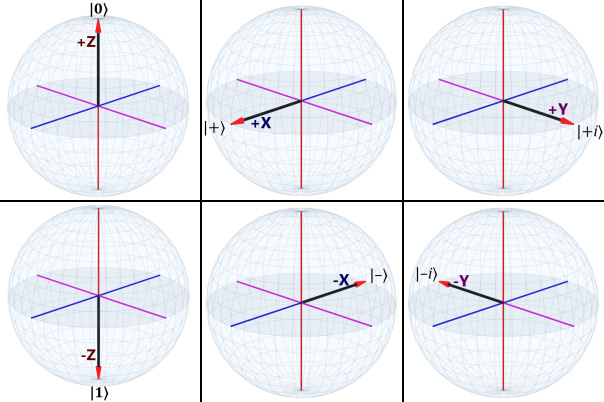
Above are the six eigenstates of the Bloch sphere. On the left, |0⟩ and |1⟩ (top and bottom); in the middle, |+⟩ and |–⟩ and on the right, |+i⟩ and |–i⟩. Each of these three pairs form an eigenbasis capable of depicting any state of the system.

If we want, we can be more explicit by labeling them (respectively): |Z+⟩, |Z-⟩ and |X+⟩, |X-⟩ and |Y+⟩, |Y-⟩ but the first versions are commonly seen.

Note that another common notation when considering spin on just the Z-axis is to use |+⟩ for |0⟩ and |–⟩ for |1⟩ because the |+⟩ and |–⟩ are more reflective of spin measurements (which have eigenvalues of plus and minus hbar-over-two — the plus and minus are the up and down spin states respectively).

The |0⟩ and |1⟩ notation is more common in quantum computing because of the similarity to classical bits, 0 and 1.

Bloch Sphere “Latitude” and “Longitude”

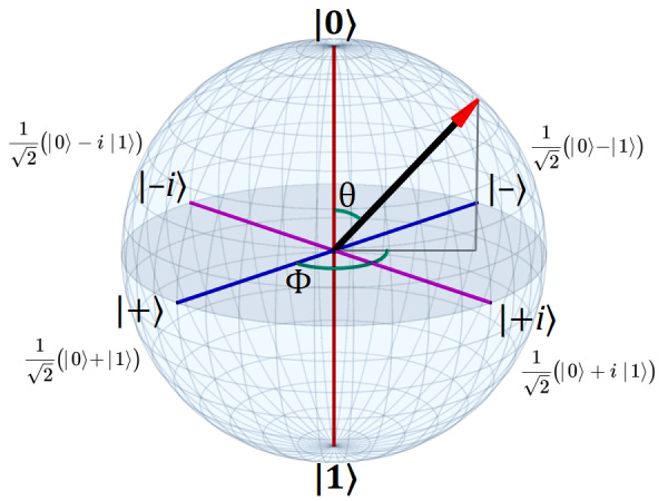
A point on a sphere can be defined by two angles: theta (θ) and phi (φ).⁷

We start with the general form of a superposition implied by the {|0⟩, |1⟩} basis:

\(|\Psi\rangle=c_1|0\rangle+c_2|1\rangle \)

Where the coefficients cₙ are complex numbers.

We can write it more explicitly as:

\(|\Psi\rangle=({a}_{1}\!+\!{ib}_{1})|0\rangle+({a}_{2}\!+\!{ib}_{2})|1\rangle\)

Where aₙ and bₙ are real numbers. This implies four degrees of freedom, but quantum mechanics requires superpositions be normalized such that:

\(|{c}_{1}|^{2}+|{c}_{2}|^{2}={1}\)

Because these coefficients are probability amplitudes, and their norm squared must sum to 1. This restricts their allowed values. For instance, if one is larger, the other must be smaller. This removes one degree of freedom.

We can then look for a suitable coordinate system having only three degrees of freedom. A useful choice is the Hopf coordinate system where:

\({c}_{1}={e}^{i\omega}\cos\frac{\theta}{2},\qquad{c}_{2}={e}^{i(\omega+\phi)}\sin\frac{\theta}{2} \)

Note the three degrees of freedom, theta (θ), phi (φ), and omega (ω) — all three are angles. (As we’ll see, the latter is a global phase angle we can ignore in quantum mechanics.)

Plugging the Hopf coordinates into the general superposition gives us:

\(|\Psi\rangle=e^{i\omega}\cos\frac{\theta}{2}|0\rangle+e^{i(\omega+\phi)}\sin\frac{\theta}{2}|1\rangle \)

Note that:

\({e}^{{i}(\omega+\phi)}={e}^{{i}\omega}e^{{i}\phi}\)

So, we can extract the global phase, omega (ω), like this:

\(|\Psi\rangle={e}^{{i}\omega}\left[\cos\frac{\theta}{2}|{0}\rangle+{e}^{{i}\phi}\sin\frac{\theta}{2}|{1}\rangle\right]\)

Because global phase isn’t physically detectable, we can ignore it, leaving:

\(|\Psi\rangle=\cos\frac{\theta}{2}|{0}\rangle+{e}^{{i}\phi}\sin\frac{\theta}{2}|{1}\rangle\)

And now we’re dealing with only two degrees of freedom, the angles theta (θ) and phi (φ). Theta is the angle relative to the |0⟩ state (the +Z-axis), and phi is the angle relative to the |+⟩ state (the +X-axis).

Note that in the Hopf coordinate system theta is restricted to the range 0°–180° while phi has the full circular range 0°–360°. Dividing theta by two effectively reduces its range to 0°–90° (which is why |0⟩ and |1⟩ are orthogonal states).

Global Phase

I sneaked a couple of fastballs over the plate regarding global phase and the Hopf coordinates, so let’s dig into that a bit more. Most references to the Hopf coordinate system define the coefficients using three distinct angles:

\({c}_{1}={e}^{{i}\phi_{1}}\cos\theta,\quad{c}_{2}={e}^{{i}\phi_{2}}\sin\theta\)

Note the two angles phi (φ), one for each coefficient. But above it’s written as:

\({c}_{1}={e}^{{i}\omega}\cos\frac{\theta}{2},\quad{c}_{2}={e}^{{i}(\omega+\phi)}\sin\frac{\theta}{2}\)

This is what allows us to factor out one of the exponentials. If we have two distinct values, call them x and y, we can always write them as x and x+n, where n=y–x.⁸

To illustrate, if x=45 and y=120, then y–x=75, so x and y can be written as 45 and 45+75. This makes x common to both, and we can factor it out.

Therefore, the second term can be rewritten:

\(|\Psi\rangle={e}^{{i}\omega}\cos\frac{\theta}{2}|{0}\rangle+{e}^{{i}\omega}{e}^{{i}\phi}\sin\frac{\theta}{2}|{1}\rangle\)

Which allows us to factor out the first exponential:

\(|\Psi\rangle={e}^{{i}\omega}\left[\cos\frac{\theta}{2}|{0}\rangle+{e}^{{i}\phi}\sin\frac{\theta}{2}|{1}\rangle\right]\)

Any quantum superposition is a linear sum of the contributing states and thus is itself a state. For any given state:

\(|\psi\rangle={e}^{{i}\phi}|\psi\rangle\)

The exponential term is the global phase, and it is not something we can measure or detect. Global phase has no physical meaning, and therefore we can ignore it. Only the relative phase between states matters.

The takeaway here is that, given any two states:

\(|\Psi\rangle={e}^{{i}\phi_{1}}|\psi_{1}\rangle+{e}^{{i}\phi_{2}}|\psi_{2}\rangle\)

We can always use the n=y–x trick to give us:

\(|\Psi\rangle={e}^{{i}\phi_{1}}|\psi_{1}\rangle+{e}^{{i}\phi_{1}}e^{{i}(\phi_{2}-\phi_{1})}|\psi_{2}\rangle\)

And then factor out the global phase leaving only the relative phase, φ₂-φ₁.

Some Examples

Let’s consider a few examples of theta and phi to see what we get.

If θ=0°:

\(\cos({0})|{0}\rangle\!+\!{e}^{{i}\phi}\sin({0})|{1}\rangle={1}|{0}\rangle\!+\!{e}^{{i}\phi}{0}|{1}\rangle=|{0}\rangle\)

Because cos(0)=1 and sin(0)=0. And because of the zero in the second term, it doesn’t matter what phi is.

If θ=180° (remember it gets divided by two, so its effective value is 90°):

\(\cos({90})|{0}\rangle\!+\!{e}^{{i}\phi}\sin({90})|{1}\rangle={0}|{0}\rangle\!+\!{e}^{{i}\phi}{1}|{1}\rangle={e}^{{i}\phi}|{1}\rangle=|{1}\rangle\)

Because cos(90)=0 and sin(90)=1. Again, phi doesn’t matter, but in this case it’s because it has become a global phase. These two states are both degenerate in terms of phi. The situation is similar to being at the North or South Pole on Earth. Your longitude becomes degenerate in terms of your location.

If θ=90° and φ=0° (remembering θ/2):

\(\cos({45})|{0}\rangle\!+\!{e}^{{i}{0}}\sin({45})|{1}\rangle=\frac{1}{\sqrt{2}}|{0}\rangle+\frac{1}{\sqrt{2}}|{1}\rangle\)

The result should be familiar as the |X+⟩ superposition shown above.

I’ll leave the other three eigenstates as exercises for the dedicated reader.

In Closing…

The Bloch sphere is handy in quantum computing, because qubits are two-state systems. The concept can extend to systems with more levels, but it becomes an object we can no longer visualize.

The most important aspect of this is that classical computing bits have a single degree of freedom with only two values. A visualization of them requires only the polar |0⟩ and |1⟩ states with no spherical surface between them.⁹

But qubits can have an infinite range of values between those states (they live in an ℝ² space rather than a ℤ₂ space), and that is part of what makes quantum computers so different and, for some applications, so powerful.

Until next time…

1. Which can be — and sometimes are — used as quantum computing qubits.

2. Which is the quantum spin of photons.

3. In fact, any two antipodal points on the sphere comprise an eigenbasis.

4. “Eigen” this and “eigen” that. The term is German for “proper”, and to some extent one can ignore it and instead think just of “states”, “vectors”, and “bases” etc.

5. A more general meaning for orthogonal is “completely independent of each other”.

6. These superpositions should look familiar from the quantum spin post.

7. Theta can be thought of a “latitude” while phi can be thought of as “longitude”.

8. Note that, if x is greater than y, then n is negative, which is fine.

9. The hardware in classical computers takes measures to ensure this.