Quantum Spin

The Bloch Sphere — very handy for depicting spin ½ systems.

Popular treatments of quantum mechanics often treat quantum spin lightly. It reminds me of the weak force, which science writers often mention only in passing as ‘related to radioactive decay’ (true). There’s an implication it’s too complicated to explain (maybe sort of true).

With quantum spin, the handwave is that it is ‘similar to classical angular momentum’ (similar to actual physical spinning objects), but different in mysterious quantum ways too complicated to explain.

Ironically, it’s one of the simpler quantum systems, mathematically.

To be fair, “simple mathematical quantum system” might have a whiff of oxymoron for many, and simple is certainly relative. That said, it’s not that bad, which is why some aspects of spin are often introduced early in quantum mechanics courses.

Note that this simplicity, and this post, concern particles with half integer spin — particles with spin ½. This includes fermions (such as electrons and quarks) and even some atoms (such as silver atoms because of their electron configuration).

What can make the topic opaque is the math prerequisites: a general grasp of complex numbers, vector spaces, linear transformations, and operators. The need for some grounding in these topics may account for why pop science writers avoid quantum spin.

Part of the problem may be that other than certain basics, there isn’t much to be said about spin besides the math. Still, those basics are interesting and worth exploring. Some college courses introduce most of what I’ll show you here in the first lecture.

Quantum spin is a lot like physical spin. The basic math for classical angular momentum, which students learned in earlier physics classes, is similar but with quantum differences:

Firstly, the current view is that nothing is physically spinning because it would have to do so faster than light.

Secondly, classical angular momentum can have any value, but spin has only two, the eigenstates, “spin-up” and “spin-down” with two respective eigenvalues, plus and minus h-bar-over-two.¹

Simple representation of a Stern-Gerlach device. An oven (left, green) produces a beam of silver atoms (red) that passes between two powerful magnets (blue). This splits the beam into two distinct beams of atoms with “spin-up” and “spin-down” eigenstates relative to the vertical axis. To measure the horizontal (or any other) axis, the device is physically rotated to the desired angle.

This result comes from the Stern-Gerlach experiment. The expectation was a fan-like spray of silver atoms with various spin values reacting to the magnetic field. Instead, the atoms formed two distinct streams, one deflected up, the other down.

Unlike energy or momentum, which can have many quantum values, spin is a strictly binary property.² That is why it’s one of the simpler quantum systems. (When talking about spin ½ particles. It gets a bit more complicated with higher spin values.)

These spin experiments demonstrate an important property of certain quantum states: they are non-commutative — the order of measurements matters.

The following series of experiments tease out this surprising difference between the classical and the quantum worlds.

Experiment #1

Figure 1. Spin test, Z-axis.

First, we need to understand a basic spin measurement.

Popular accounts and lectures sometimes invoke a magic box that tests familiar properties such as hard/soft or black/white. I’m going to skip that and use a magic box that measures spin.

Not so magic, because Stern-Gerlach devices are real and work as described. These experiments have been done, and they confirm quantum predictions.

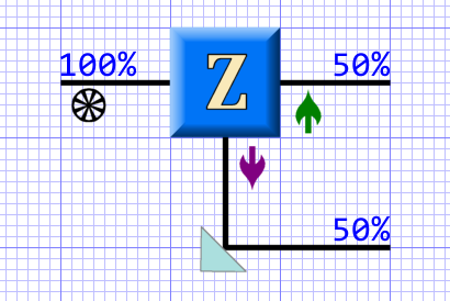
Figure 1 shows a schematic of a single spin test. Particles enter the box from the left and exit right or down depending on their measured spin (up or down, as indicated by the arrows). The “Z” means this box measures the Z-axis (canonically the vertical axis). A reflector diverts the spin-down particles to the right (you’ll see why below).

The 100% on the left indicates that all particles enter the box. The wheel shape below it symbolizes that the particles have unknown — and presumably evenly distributed — spins.

For now, I’m ignoring the notion that unmeasured particles even have a distinct spin. Quantum mechanics suggests they do not.

Given the presumed even distribution (or that spin is undetermined), over time we expect an equal mix of up and down measurements. And that’s what we find: 50% turn out to be spin-up; 50% turn out to be spin-down. (The blue numbers on the right reflect this fact.)

Note that we can rotate the box (along its long axis) to measure any angle. If we do, we always get a 50/50 mix of spin-up and spin-down relative to the chosen axis.

More importantly, note that our measurement puts the particle in a known spin state in a process called wavefunction reduction (or collapse), and that this reduction to a known state presents one of the greatest mysteries in quantum mechanics. For details see:

The Vexing Problem of Wavefunction Collapse

Quantum Spin States

There are many ways authors depict spin states. Shown below are several ways of notating the same state depending on what the author wants to say.

For the spin-up state:

\(|up\rangle=|{+}\rangle=|{0}\rangle=|Z_{+}\rangle=\begin{bmatrix}{1}\\{0}\end{bmatrix}\)

And for the spin-down state:

\(|down\rangle=|{-}\rangle=|{1}\rangle=|Z_{-}\rangle=\begin{bmatrix}{0}\\{1}\end{bmatrix}\)

The first version is a casual (but evocative) notation. The second and third are the most common from what I’ve seen. The fourth is explicit about which axis is involved. That can be helpful when dealing with multiple axes in one equation. The fifth is the column vector for the eigenstate actually used in calculations.

If the notation above is mysterious, see:

Bra-Ket Notation

Remember that any measurement of a quantum system involves eigenstates (aka eigenvectors) that represent the possible outcomes. Both the spin-up and spin-down results are such eigenstates. And they are the only possible outcomes of a measurement on a spin ½ particle.

We view a particle with an unknown spin as a superposition of the two orthogonal spin eigenstates. We can write this as:

\(\psi=\alpha\!\mid\!{0}\rangle+\beta\!\mid\!{1}\rangle\)

Where α (alpha) and ß (beta) are complex coefficients representing the probability of getting that measurement. In a particle with unknown spin, we have no way to actually know these coefficients.

However, in an even distribution of spins over many measurements, we know experimentally the outcomes divide equally, so we know that in the general case we have:

\(\mid\!\Psi\rangle\;=\;\frac{1}{\sqrt{2}}\!\mid\!{0}\rangle+\!\frac{1}{\sqrt{2}}\!\mid\!{1}\rangle\;=\;\frac{\mid{0}\rangle\,+\mid{1}\rangle}{\sqrt{2}}\)

The actual probability is the norm squared of the coefficients, and:

\(\left|\frac{1}{\sqrt{2}}\right|^{2}=\frac{1}{2},\qquad\frac{1}{2}+\frac{1}{2}={1}\)

A measurement always has some outcome, so the probabilities always must sum to 1.

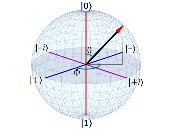
This applies to any angle we measure, but the Z-axis, the vertical axis, is the canonical basis. As such, we assign the |0⟩ (“ket zero”) eigenstate to a spin-up measurement on that axis and the |1⟩ (“ket 1”) state to the spin-down measurement.

We call this the {|0⟩, |1⟩} eigenbasis, and this basis spans all possible spin states, including those on other axes.

This is an important point. Particles with spin ½ have three orthogonal axis, X, Y, and Z. One might think we also need an eigenbasis for the other two axes. We do not. The {|0⟩, |1⟩} basis spans all possible spin states.

We represent those other axes as quantum superpositions of the basis states.

For the X-axis:

\(\mid\!{X_+}\rangle\!=\mid\!{+}\rangle=\frac{\mid{0}\rangle\;+\;\mid{1}\rangle}{\sqrt{2}},\qquad\mid\!{X_-}\rangle\!=\mid\!{-}\rangle=\frac{\mid{0}\rangle\;-\;\mid{1}\rangle}{\sqrt{2}} \)

The more formal (less ambiguous) labels are |X+⟩ and |X-⟩, but they are often labeled as |+⟩ and |-⟩, respectively.

For the Y-axis:

\(\mid\!{Y_+}\rangle=\mid\!{i_+}\rangle=\frac{\mid{0}\rangle\;+\;{i}\mid{1}\rangle}{\sqrt{2}},\qquad\mid\!{Y_-}\rangle=\mid\!{i_-}\rangle=\frac{\mid{0}\rangle\;-\;{i}\mid{1}\rangle}{\sqrt{2}}\)

The more formal labels are |Y+⟩ and |Y-⟩, but (because of the imaginary axis involved) these are often labeled |i+⟩ and |i-⟩.

In both cases, note the minus signs in the spin-down states. That is their only difference from the spin-up states. These three orthogonal basis axes are called out on the image (the Bloch sphere) at the top of this post.³

To repeat an earlier important point: After a measurement we know the spin state. The state vector has jumped (“collapsed”) to that state. If, for instance, we had measured spin-up, the quantum state is now just:

\(\psi=\mid\!{0}\rangle\qquad\dots\textsf{or}\ldots\qquad\psi={1.0}\mid\!{0}\rangle+{0.0}\mid\!{1}\rangle\)

Further measurements return the same result with 100% probability.

Experiment #2

Which brings us to the next experiment. This involves three Z-boxes, all performing the same test of spin on the Z-axis:

Figure 2. Again, the blue percentages show how many particles exit a box given all that enter. The red percentages (far right) show how many particles exit the entire process (and these must sum to 100% because none are lost).

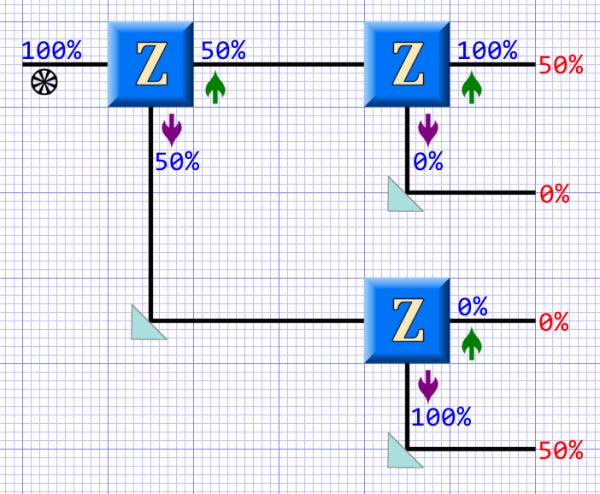
The outputs from the first test are funneled to second tests which repeat the Z-axis test.⁴ This experiment shows the first test putting the particles into known eigenstates such that further immediate tests on the particle have a 100% chance of giving the same results. (Unlike the first where it was 50% each.)

We see a similar thing with photons and polarizing filters. A photon that passes through a vertical polarizer is now vertically polarized and passes through a second vertical filter with 100% probability.

This, so far, seems almost classical behavior, as long as we accept that we’ve changed the state of the particles. (The second tests merely reenforce or refresh that change.)

Experiment #3

Now let’s try measuring a different axis in the second test. We’ll measure the X-axis second:

Figure 3. Measuring the X-axis after measuring the Z-axis. We’re discarding the particles with spin-down in the first test. If we did send them through an X-axis test, that test would also produce 50/50 results.

With spin, orthogonal axes are not correlated, and since we know the value of the Z-axis measurement, we can know nothing about the state of spin on the X-axis (or the Y-axis).⁵

It’s not merely our ignorance; the spin state on the X-axis is undetermined.

Because the particle is now in a known eigenstate, |0⟩ on the Z-axis, spin on the two orthogonal axes is an equal superposition of possible results on those axes (as shown above). As such, we expect 50/50 results over multiple tests.

The X-axis measurement here implies another basis, usually written as {|+⟩, |-⟩}, but, as shown above, defined in terms of the eigenbasis {|0⟩, |1⟩}:

\(\mid\!X_+\rangle=\frac{\mid{0}\rangle\;+\;\mid{1}\rangle}{\sqrt{2}},\qquad\mid\!X_-\rangle=\frac{\mid{0}\rangle\;-\;\mid{1}\rangle}{\sqrt{2}}\)

We can just as easily consider X-axis the primary basis and then define the Z-axis (and Y-axis) as superpositions of the {|+⟩, |-⟩} basis. We could do the same with the Y-axis.

Note that we’re seeing quantum behavior in the sense that knowing the spin state of the one axis makes the spin state of the other axes undetermined. These orthogonal measurements do not commute — they are incompatible.

The last experiment drives this point home.

Experiment #4

This experiment starts off the same way as the previous one, but adds a third test, another Z-axis test. Above we saw that repeating a test of the same axis gave the same result. But here…

Figure 4. Three tests, Z-X-Z. (Ignoring spin-down particles in first two)

We see that the third test has a 50/50 split of particles (just as the first one did). This is because the second test destroyed our knowledge of the first result. This is implicit in the definition of the |X+⟩ state:

\(\mid\!X_+\rangle=\frac{\mid{0}\rangle\;+\;\mid{1}\rangle}{\sqrt{2}}\)

The state is an equal superposition of the |0⟩ and |1⟩ states (just as it was before the first test).

We’ve Only Just Begun

This only scratches the surface. The main point is that knowing the spin state on a given axis means the spin state of the other orthogonal axes is a fully undetermined superposition of possible outcomes, each with 50/50 odds.

If we measure a non-orthogonal axis, we see a correlation that depends on the angle. The superposition then looks like:

\(\psi=\cos^{2}\theta\mid\!{0}\rangle+\sin^{2}\theta\mid\!{1}\rangle\)

Where θ (theta) is the angle relative to |0⟩ (the +Z axis). The closer that angle, the higher the probability of getting the |0⟩ result. Larger angles make the |1⟩ result more probable.

Lastly, recognize that, not only are orthogonal spin measurements not compatible — knowing spin on a measured axis erases our knowledge of all other axes — but also non-commutative. The order of measurements determines the outcome.

This is a key aspect (some say the key aspect) of the quantum world. It’s embodied in the Heisenberg Uncertainty Principle.

For more info, see:

The Heisenberg Uncertainty Principle

Next time I’ll talk more about quantum states and explain the Bloch sphere.

1. If there is an interest, I can write about eigenstates and eigenvalues (and eigenvectors and eigenbases).

2. Which is why half-integer spin particles are one way to create quantum computing qubits.

3. More on that blue sphere next week!

4. The reflector redirects the streams to the right for the sake of the diagrams but wouldn’t exist in a real experiment because it would affect the particle spins.

5. This is similar to how knowing a particle’s precise momentum means we know nothing about its location (and vice versa).